Built-in Functions

Flitter supports the following built-in functions.

Vector utility functions

accumulate( xs )

Return a vector with the same length as xs formed by adding each value to an accumulator starting at 0.

count( xs , ys )

Return a vector with the same length as xs containing the number of times each of the elements in xs occurs in ys.

len( xs )

Return the length of vector xs.

max( x [ , … ] )

Return the maximum value in the vector x with one argument, or the largest of the arguments in vector sort order.

maxindex( x [ , … ] )

Return the index of the maximum value in the vector x with one argument, or the index of the largest argument in vector sort order (with the 1st argument being index 0).

mean( xs [ , w=1 ] )

Return a numeric vector, of length w, obtained by summing together w-element groups of xs, i.e., xs[0..w] + xs[w..2*w] + xs[2*w..3*w] + …, up to the end of xs with the final group truncated if necessary, and then dividing by the number of elements contributing to each value. mean() of an empty vector is w inf values. mean() of a non-numeric vector, or with w non-numeric or less than 1, is null. Equivalent to sum(xs, w) / sum(1[..len(xs)], w).

min( x [ , … ] )

Return the minimum value in the vector x with one argument, or the smallest of the arguments in vector sort order.

minindex( x [ , … ] )

Return the index of the minimum value in the vector x with one argument, or the index of the smallest argument in vector sort order (with the 1st argument being index 0).

product( xs [ , w=1 ] )

Return a numeric vector, of length w, obtained by multiplying together w-element groups of xs, i.e., xs[0..w] * xs[w..2*w] * xs[2*w..3*w] * …, up to the end of xs with the final group truncated if necessary. product() of an empty vector is w ones. product() of a non-numeric vector, or with w non-numeric or less than 1, is null.

shuffle( source , xs )

Return the shuffled elements of xs using the pseudo-random source (which should be the result of calling uniform(...)).

sum( xs [ , w=1 ] )

Return a numeric vector, of length w, obtained by summing together w-element groups of xs, i.e., xs[0..w] + xs[w..2*w] + xs[2*w..3*w] + …, up to the end of xs with the final group truncated if necessary. sum() of an empty vector is w zeros. sum() of a non-numeric vector, or with w non-numeric or less than 1, is null

zip( xs , ys [ , … ] )

Return a vector formed by interleaving values from each argument vector; for m arguments the resulting vector will be n * m elements long, where n is the length of the longest vector; short arguments will repeat, so zip(1;2;3;4, 0) == (1;0;2;0;3;0;4;0).

Mathematical functions

abs( x )

Return absolute value of x (ignoring sign).

acos( x )

Return arc-cosine (in turns not radians) of x.

angle( x ; y ) (or angle( x , y ))

Return the angle (in turns) of the cartesian vector x,y (angle(polar(th)) == th, equivalent of atan2(y, x) in other languages).

asin( x )

Return the arc-sine (in turns) of x.

ceil( x )

Return the smallest integer number larger than x.

clamp( x, y, z )

Clamp x to be no less than y and no greater than z. This function generalises to n-vectors, returning a vector the length of the longest of x, y and z, and repeating items from any of the vectors as necessary.

cross( x, y )

Compute the cross product of two 3-vectors.

cos( x )

Return cosine of x (with x expressed in turns).

dot( x, y )

Compute the dot product of two n-vectors. This is the equivalent of sum(x * y).

exp( x )

Return \(e\) raised to the power of x.

floor( x )

Return the largest integer number smaller than x.

fract( x )

Return fractional part of x (equivalent to x - floor(x)).

hypot( x [, …] )

Return the square root of the sum of the square of each value in x with one argument, with multiple arguments return a vector formed by calculating the same for the 1st, 2nd, etc., element of each of the argument vectors.

length( x ; y ) (or length( x , y ))

Return the length of the cartesian vector x,y. This is similar to hypot() but restricted to cartesian vectors. The difference is that it will accept an n-vector of x,y pairs in the first form and return a sequence composed of the length of each pair, while hypot() will return the length of a single n-dimensional vector. This function is designed to be used with angle() to convert cartesian coordinates into polar coordinates.

log( x )

Return natural logarithm (\(log_e\)) of x (log(exp(x)) == x)

log2( x )

Return \(log_2\) of x.

log10( x )

Return \(log_{10}\) of x.

map( x , y , z )

Map a value of x in the range [0,1] into the range [y,z]; equivalent to (1-x)*y + x*z (including in n-vector semantics). Values of x outside of the range [0,1] will result in values outside of the range [y,z]. Use clamp() or linear() on x if the range is to be restricted.

normalize( x )

Return x / hypot(x).

polar( th )

Return the unit cartesian pair x;y matching the angle th (expressed in turns) – equivalent to zip(cos(th), sin(th)).

round( x )

Return x rounded to the nearest integer number, with 0.5 rounding up.

sin( x )

Return sine of x (with x expressed in turns).

sqrt( x )

Return the square root of x.

tan( x )

Return the tangent of x (with x expressed in turns).

Quaternion functions

Quaternions are 4-vectors, w;x;y;z, that can be used to describe an arbitrary rotation in 3-dimensional Cartesian space. The identity quaternion is 1;0;0;0.

qbetween( u , v )

Return the quaternion representing a rotation of the vector u to point in the direction of the vector v.

qmul( p , q )

Return the product of the quaternion p and the quaternion q, which is equivalent to the rotation q followed by the rotation p.

quaternion( axis , turns )

Return a Euler-rotation unit-quaternion representing a turns rotation around the axis vector (clockwise looking in the direction of the vector).

slerp( t , p , q )

Return the quaternion spherical linear interpolation between p and q with t=0 representing p and t=1 representing q. Values of t in the range [0,1] will smoothly interpolate between the rotations p and q – equivalent to sweeping the arc between the points p and q on a sphere. Values of t outside of this range will continue along this arc beyond p and q, eventually circling round to rejoin the arc from the other side.

Matrix functions

Matrices are either 9- or 16-vectors, in column-major order, representing a 3x3 or 4x4 matrix. There are a few places where matrices are supported, such as the matrix attribute of a 3D !transform node.

inverse( M )

Returns the matrix inverse of a 3x3 or 4x4 matrix.

point_towards( direction, up )

Returns a 4x4 matrix representing a rotation making the Z-axis point towards direction and the Y-axis point towards up, where both of these are 3-vectors. If up is not orthogonal to direction then the Z-axis takes precedence and the Y-axis will be aligned as closely to up as possible.

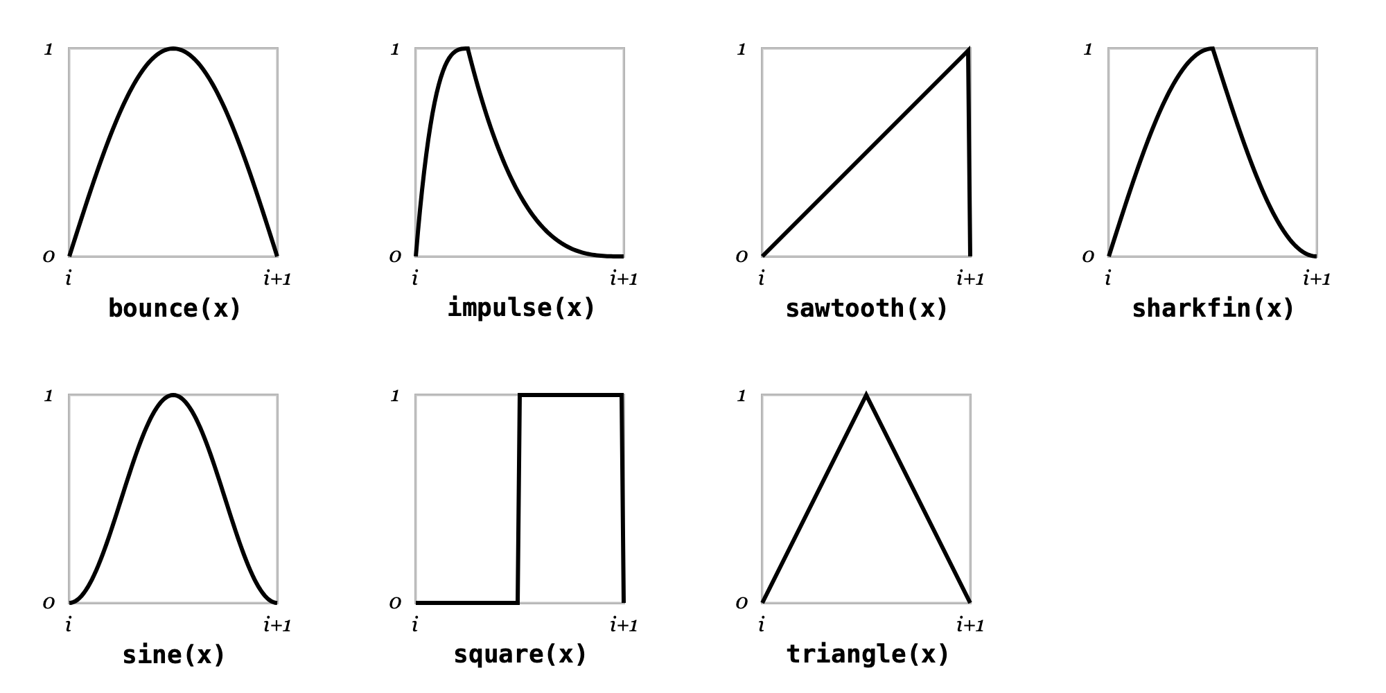
Waveform functions

All of the waveform functions return a repeating wave in the y range [0,1] with one wave per unit of x.

bounce( x )

A wave akin to a bouncing ball made up of half of a sine wave.

impulse( x [ , c=0.25 ] )

A cubic rising and falling wave with the high point at c.

sawtooth( x )

A rising sawtooth wave function.

sharkfin( x )

A “shark fin” wave function made up of two quarter parts of a sine wave.

sine( x )

A sine wave shifted so that it begins and ends at 0.

square( x )

A square wave with the rising edge at 0.5.

triangle( x )

A symmetric triangle wave function.

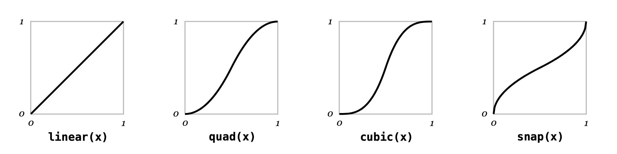
Easing functions

The “easing” functions map from x in the range [0, 1] to a y in the range [0, 1], with values of x less than 0 returning 0 and values greater than 1 returning 1.

cubic( x )

A cubic easing function.

linear( x )

A linear easing function.

quad( x )

A quadratic easing function.

snap( x )

A square-root easing function (conceptually a quadratic easing function with the x and y axes flipped).

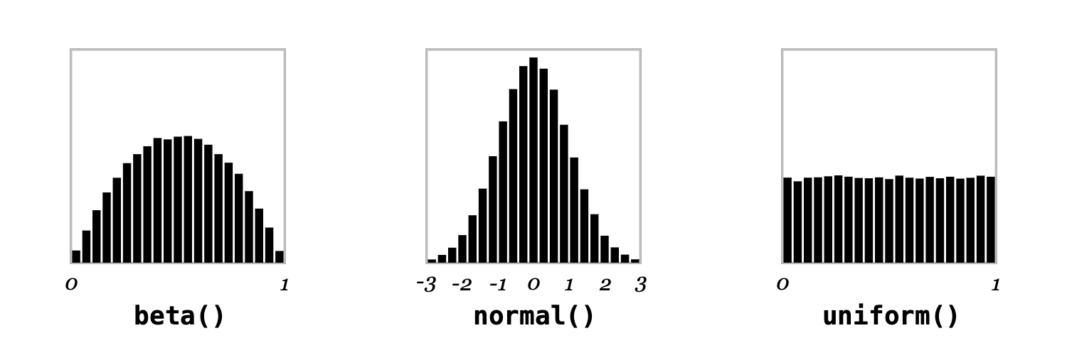
Pseudo-random functions

Flitter provides three useful sources of pseudo-randomness. These functions return special “infinite” vectors that may only be indexed. These infinite vectors provide reproducible streams of pseudo-random numbers.

beta( [ seed ] )

A Beta(2,2) distribution pseudo-random source.

normal( [ seed ] )

A Normal(0,1) distribution pseudo-random source. The output range is notionally unbounded, but in practice limited by the resolution of the algorithm to \(\pm 9.4193\).

uniform( [ seed ] )

A Uniform(0,1) distribution pseudo-random source.

The single argument to all of the functions is a vector that acts as the pseudo-random seed. Floating-point numbers within this seed vector are floor-ed to integer numbers before the seed is calculated. This is to allow new seeds to be easily generated at intervals, e.g.: uniform(:foo;beat) will create a new stream of pseudo-random numbers for each beat of the main clock. Multiplying or dividing this seed value then allows for different intervals, e.g., four times a beat: uniform(:foo;beat*4).

Pseudo-random streams can be indexed with a range vector to generate a vector of numbers, e.g.: uniform(:some_seed)[..100] will generate a 100-vector of uniformly distributed numbers. Streams are very long (see note below) and are unit-cost to index – so indexing the billionth number takes the same amount of time as the first. Negative indices wrap around to the end of the stream.

Streams are considered to be true in conditional expressions (if, and, etc.). In all other aspects, they behave like the null vector, e.g., attempts to use them in mathematical expressions will evaluate to null.

For example:

let SIZE=1280;720

!window size=SIZE
    !canvas
        for i in ..10
            let x=uniform(:x;beat)[i] y=uniform(:y;beat)[i]
                r=2*beta(:r;beat)[i] h=uniform(:h;beat)[i]
            !path
                !ellipse point=(x;y)*SIZE radius=r*50
                !fill color=hsv(h;1;1)

This will create 10 circles distributed uniformly around the window with different radii clustered around 50 pixels and different uniformly picked hues. Every beat, the circles will be drawn in different places and with different sizes and hues. Note the use of symbols (:x, :y, etc.) combined with beat to create unique seeds and then indexing with the i counter to generate individual items from these streams. This code will draw exactly the same sequence of circles every time it is run, as the pseudo-random functions are stable on their seed argument. There is no mechanism for generating true random numbers in Flitter.

Pseudo-random streams may be bound to a name list in a let expression to pick off the first few values, e.g.:

let x;y;z = uniform(:position)

There is little difference in pseudo-randomness between selecting a new seed and selecting a different index. The example above could be written equivalently as:

let SIZE=1280;720

!window size=SIZE
    !canvas
        for i in ..10
            let x;y;h=uniform(:x;i;beat)
                r=2*beta(:r;beat)[i]
            !path
                !ellipse point=(x;y)*SIZE radius=r*50
                !fill color=hsv(h;1;1)

This creates a new uniform distribution for each circle and beat, and then pulls three values from it. Note that r is still set by indexing a single stream per beat, as a single name let will bind the whole sequence rather than an item from it. There is a slight performance benefit in reading large numbers of values from a single sequence over reading a small number of values from a large number of sequences.

Note

The uniform() and normal() streams have an internal index range of \([0, 2^{64})\) and beta() streams have an internal index range of \([0, 2^{62})\). However, as all numbers in Flitter are double-precision floating points, the actual index range is in practice limited by the safe integer range of double-precision: \((-2^{53}, 2^{53})\). As the internal range is significantly larger than this, the negative portion of the safe range (which maps to the end of the internal range) does not overlap with the positive portion.

Noise functions

noise( seed , x [ , y [ , z [ , w ] ] ] ] )

OpenSimplex 2S noise function

• seed is a seed value, as per Pseudo-random sources

• x is the first dimension

• y is an optional second dimension

• z is an optional third dimension

• w is an optional fourth dimension

The function returns a value in the range (-1,1). The function can be thought of as creating a wiggly line in 1 dimension, a landscape with hills and dips in 2 dimensions, a volume of space filled with clouds in 3 dimensions and is probably hard for most people to conceptualize in 4 dimensions.

A slice through 4D noise will look like a 3D noise function, a slice through 3D noise will look like the output of a 2D noise function and, similarly, a slice through 2D noise will look like the output of a 1D noise function. Often a useful thing to do is to use a value derived from the beat counter as one of the inputs, yielding a 1D, 2D or 3D noise function that will smoothly change over time for the same input space.

The function is entirely deterministic - always producing the same output for the same inputs. The seed value should be used to create multiple independent noise sources.

Multi-value vector inputs

If one of the x, y, z or w arguments is a vector longer than 1, then the function will return a multi-value output. The return value is equivalent to the code:

(((noise(seed, ix, iy, iz, iw) for iw in w) for iz in z) for iy in y) for ix in x

However, calling noise() with an n-vector is significantly faster than n separate calls.

Multi-octave noise

It is often useful to layer a number of noise functions on top of each other with different scales and weights to produce a more complex surface - this is particularly useful when attempting to produce organic looking results.

For example:

let n = 4
    scale = 1;2;4;8
    weight = 1;0.5;0.25;0.125
    total = sum(weight)
    z = (noise(:seed;i, x*scale[i], y*scale[i])*weight[i] for i in ..n) / total

Here the scale of the inputs doubles with each iteration and the weight halves.

Flitter provides a function that will do this calculation significantly faster than the equivalent code:

octnoise( seed , n , k , x [ , y [ , z *[ , w ] ] ] ] )

Multi-octave OpenSimplex 2S noise function

• seed is a seed value

• n is the number of octaves

• k is a weight constant

• x is the first dimension

• y is an optional second dimension

• z is an optional third dimension

• w is an optional fourth dimension

For each octave iteration (from \(0\) to \(n-1\)), the individual weight is computed as \(k^{-i}\) and the scaling factor for the inputs as \(2^i\). A unique seed value for each iteration is derived automatically from seed.

The equivalent octnoise() call to the code above would be:

let z = octnoise(:seed, 4, 0.5, x, y)

Again, this function will accept n-vectors as inputs and this should be done when large numbers of related noise values are required.

The particular implementation of OpenSimplex 2S noise used in Flitter is based on a Python implementation written by A. Svensson and licensed under the MIT license.

Color functions

colortemp( t [, normalize=false ] )

Return a 3-vector of R, G and B linear sRGB values for an approximation of the irradiance of a Planckian (blackbody) radiator at temperature t, scaled so that colortemp(6503.5) (the sRGB whitepoint correlated colour temperature) is close to 1;1;1 (luminance 1). The approximation only holds within the range [1667,25000] and, strictly speaking, values below 1900°K are outside the sRGB gamut. Irradiance is proportional to the 4th power of the temperature, so the values are very small at low temperatures and become significantly larger at higher temperatures; if the optional normalize parameter is true then all returned colors will instead be normalized to have luminance 1.

hsl( h ; s ; l )

Return a 3-vector of R, G and B in the range [0,1] from a 3-vector of hue, saturation and lightness (also in the range [0,1]).

hsv( h ; s ; v )

Return a 3-vector of R, G and B in the range [0,1] from a 3-vector of hue, saturation and value (also in the range [0,1]).

oklab( L ; a ; b )

Return a 3-vector of R, G and B linear sRGB values converted from Oklab L, a and b values. Lightness L is a value in the range [0,1]. The a and b coordinates are notionally unbounded but generally have a useful range of (-0.4,+0.4). The R, G and B values returned may be less that 0 or greater than 1 for colors that are not representable in linear sRGB.

oklch( L ; C ; h )

Return a 3-vector of R, G and B linear sRGB values converted from the Oklab cylindrical coordinates L, C and h. Hue h is in turns, i.e., is in the range [0,1) and wraps around. This function is equivalent to oklab(L;C*polar(h)).

Text functions

chr( o )

Return the Unicode character identified by the ordinal number o. If o is a multi-element vector then the result will be the Unicode string formed by concatenating each character. The value(s) of o is/are rounded down if not integer.

ord( c )

Return the ordinal number of Unicode character c (interpreted as a string). If c evaluates to a multi-character string then a vector of the ordinal number of each character will be returned.

split( text , [ separator="\n" ] )

Return a vector formed by splitting the string text at each instance of separator, which may be a multiple character Unicode string and which is not included in the result strings. Empty values are stripped from the end (i.e., trailing sequences of separator are ignored).

ord() and chr() can be used together with indexing to isolate a specific character range from a string. For example:

let s = "Hello world!"
    c = chr(ord(s)[4..7])

The name c will have the value "o w".

File functions

csv( filename , row )

Return a vector of values obtained by reading a specific row (indexed from 0) from the Unicode CSV file with the given filename; numeric-looking columns in the row will be converted into numeric values, anything else will be a Unicode string.

glob( pattern )

Return an n-vector of strings representing file paths matching the given shell “glob” pattern. Files are matched relative to the directory containing the running program.

read( filename )

Returns a single string value containing the entire text of filename.

read_bytes( filename )

Returns a numeric vector value containing the entire byte contents of filename as a vector of numbers in the range \([0,255]\). This is a very memory-inefficient function as each byte will be inflated to a double-precision floating point value (8 bytes).

Note

The csv, read and read_bytes functions intelligently cache the results of the read for performance, but will respond immediately to the file changing (as detected by a change to the file modification time).

Texture sampling

The sample function allows reading colors from the previous rendered image of a referenced window node. See the explanation of the !reference node for more information on references.

sample( id , coordinates [ , default ] )

Given the id of a window node and a 2n-vector of X/Y coordinates in the [0,1) range, return a 4n-vector of RGBA color values. These color values may be outside of the normal [0,1) range if the colorbits depth of the node is greater than 8. If (any of) the coordinates are outside of the [0,1) range then the returned color will either be 0;0;0;0 or default if specified (and a 4-vector).

Warning

Use of the sample function can cause a significant slow-down in the execution of the engine, as reading from a texture stalls execution until the GPU has completed rendering the previous pipeline.